It is a data driven approach
It is about learning
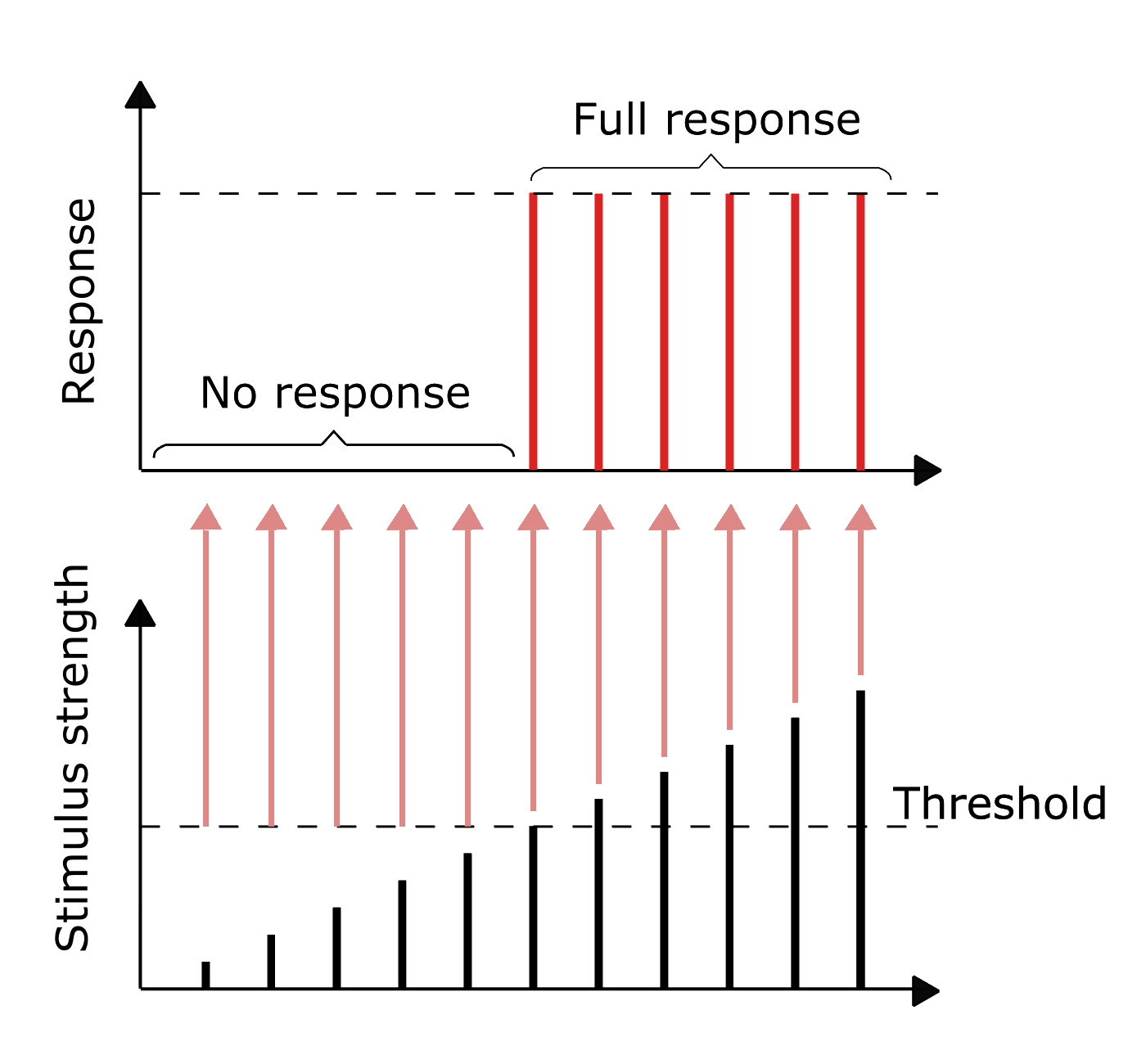
i.e. strengthening pathways
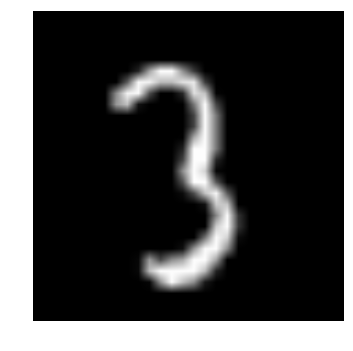
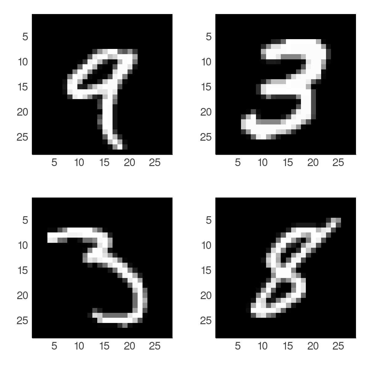
Example in image recognition:
Rather than coding all the possible ways—pixel by pixel—that a picture can represent an object, examples of image/label pairs are fed to a neural network
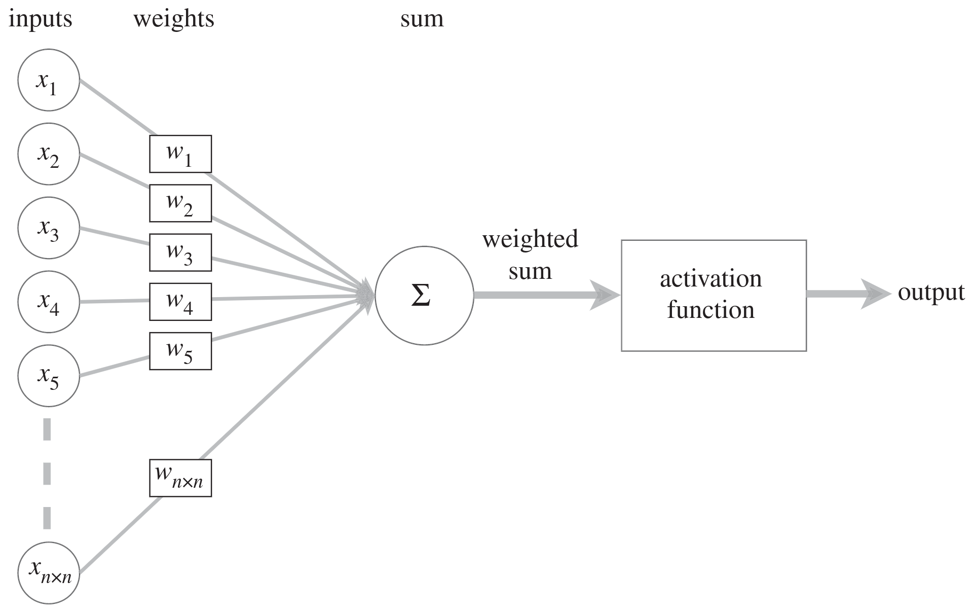
Machine learning
Computer programs whose performance at a task improves with experience
They adjust the weights and biases in an iterative manner
Supervised learning
Training set of example input/output \((x_i, y_i)\) pairs
Goal:
If \(X\) is the space of inputs and \(Y\) the space of outputs, find a function \(h\) so that
for each \(x_i \in X\), \(h_\theta(x_i)\) is a predictor for the corresponding value \(y_i\) (\(\theta\) represents the set of parameters of \(h_\theta\))
→ i.e. find the relationship between inputs and outputs
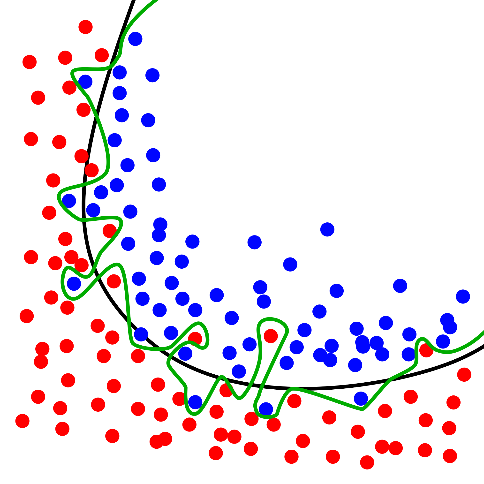
Regularization by adding a penalty to the loss function
Early stopping
Increase depth (more layers), decrease breadth (less neurons per layer) → less parameters overall, but creates vanishing and exploding gradient problems
Neural architectures adapted to the type of data → fewer and shared parameters (e.g. convolutional neural network, recurrent neural network)
Convolutional neural network (CNN)
Used for spatially structured data (e.g. image recognition)
Fully connected layer: each neuron receives input from every element of the previous layer. Images have huge input sizes and would require a very large number of neurons.
Convolutional layer: neurons receive input from a subarea (local receptive field) of the previous layer. Cuts the number of parameters.
–
Pooling (optional): combines the outputs of neurons in a subarea to reduce the data dimensions. The stride dictates how the subarea is moved across the image. Max-pooling uses the maximum for each subarea.
Both most often used through their Python interfaces
Julia’s syntax is well suited for the implementation of mathematical models
GPU kernels can be written directly in Julia
Julia’s speed is attractive in computation hungry fields
→ Julia has seen the development of many ML packages
Some of the ML packages in Julia
Flux.jl
: a machine learning stack Knet.jl
: a deep learning framework TensorFlow.jl
: wrapper for TensorFlow Turing.jl
: for probabilistic machine learning MLJ.jl
: framework to compose machine learning models ScikitLearn.jl
: implementation of the scikit-learn API
\[\text{ for }i=1,…,K\text{ and }\mathbf{z}=(z_1,…,z_K)\in\mathbb{R}^K\]
(\(\mathbb{R}\) represents the set of real numbers)
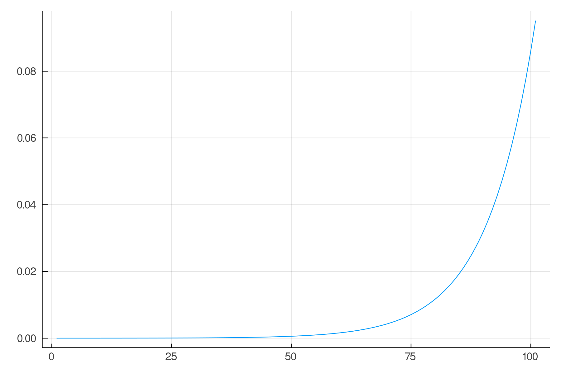
Normalizes a vector of real numbers
into a vector of numbers between 0 and 1 which add to 1
Softmax activation function
In Flux: softmax()
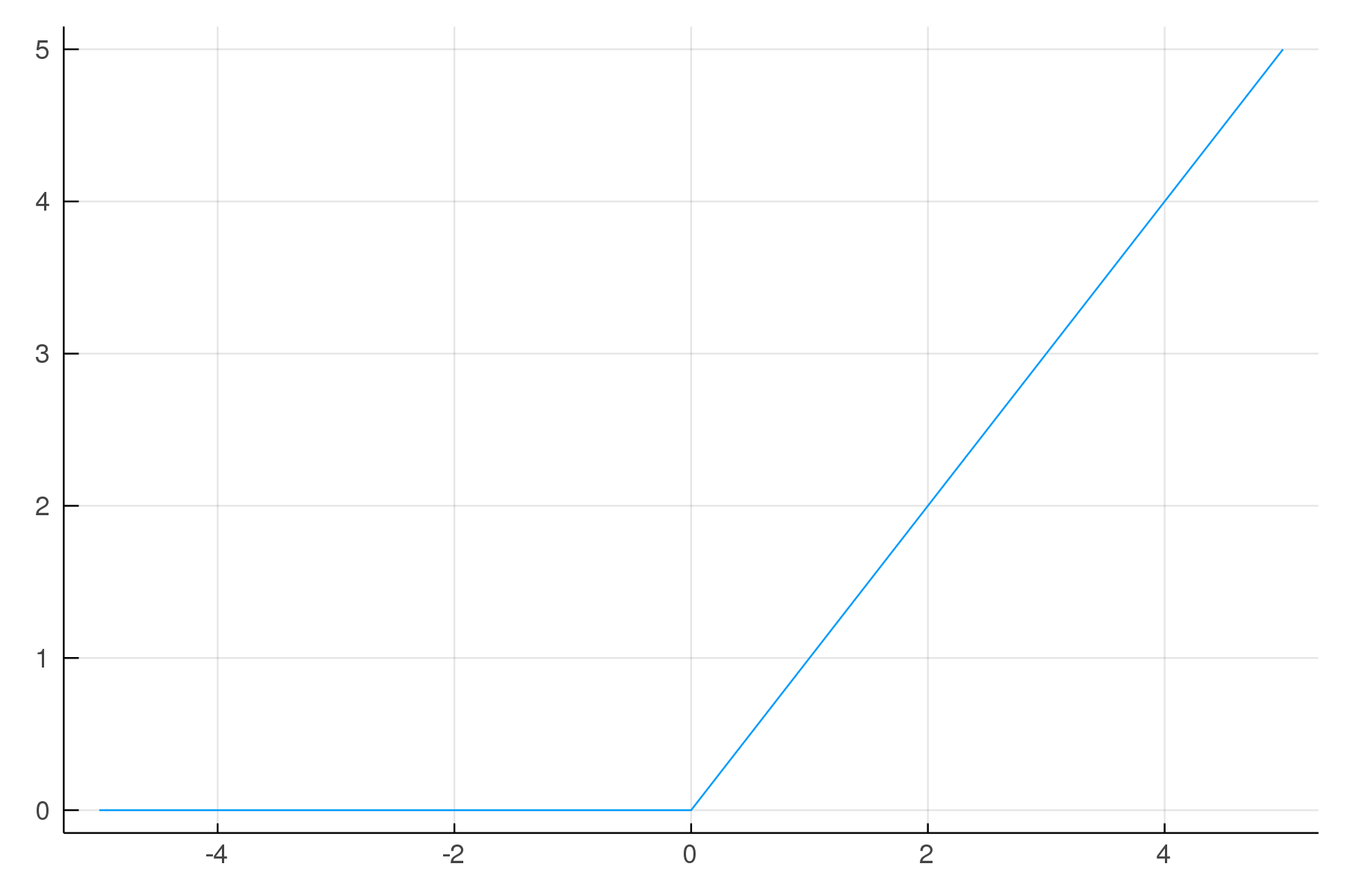
[In]
plot(softmax(-5.0:0.1:5.0))
[Out]
Multi-layer perceptron from Model Zoo
using Flux, Statistics
using Flux.Data: DataLoader
using Flux: onehotbatch, onecold, logitcrossentropy, throttle, @epochsusing Base.Iterators: repeated
using Parameters: @with_kw# using CUDAapiusing MLDatasets
# if has_cuda()# @info "CUDA is on"# import CuArrays# CuArrays.allowscalar(false)# end@with_kwmutable structArgs
η::Float64 = 3e-4# learning rate
batchsize::Int = 1024# batch size
epochs::Int = 10# number of epochs
device::Function = gpu # set as gpu, if gpu availableendfunction getdata(args)
# Loading Dataset
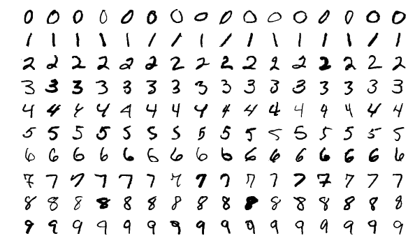
xtrain, ytrain = MLDatasets.MNIST.traindata(Float32)
xtest, ytest = MLDatasets.MNIST.testdata(Float32)
xtrain = Flux.flatten(xtrain)
xtest = Flux.flatten(xtest)
# One-hot-encode the labels
ytrain, ytest = onehotbatch(ytrain, 0:9), onehotbatch(ytest, 0:9)
# Batching
train_data = DataLoader(xtrain, ytrain, batchsize=args.batchsize, shuffle=true)
test_data = DataLoader(xtest, ytest, batchsize=args.batchsize)
return train_data, test_data
endfunction build_model(; imgsize=(28,28,1), nclasses=10)
return Chain(
Dense(prod(imgsize), 32, relu),
Dense(32, nclasses))
endfunction loss_all(dataloader, model)
l = 0f0for (x,y) in dataloader
l += logitcrossentropy(model(x), y)
end
l/length(dataloader)
endfunction accuracy(data_loader, model)
acc = 0for (x,y) in data_loader
acc += sum(onecold(cpu(model(x))) .== onecold(cpu(y)))*1 / size(x,2)
end
acc/length(data_loader)
endfunction train(; kws...)
# Initializing Model parameters
args = Args(; kws...)
# Load Data
train_data,test_data = getdata(args)
# Construct model
m = build_model()
train_data = args.device.(train_data)
test_data = args.device.(train_data)
m = args.device(m)
loss(x,y) = logitcrossentropy(m(x), y)
## Training
evalcb = () -> @show(loss_all(train_data, m))
opt = ADAM(args.η)
@epochs args.epochs Flux.train!(loss, params(m), train_data, opt, cb = evalcb)
@show accuracy(train_data, m)
@show accuracy(test_data, m)
end
cd(@__DIR__)
train()
CNN from Model Zoo
using Flux, Flux.Data.MNIST, Statistics
using Flux: onehotbatch, onecold, logitcrossentropy
using Base.Iterators: partition
using Printf, BSON
using Parameters: @with_kw# using CUDAapi# if has_cuda()# @info "CUDA is on"# import CuArrays# CuArrays.allowscalar(false)# end@with_kwmutable structArgs
lr::Float64 = 3e-3
epochs::Int = 20
batch_size = 128
savepath::String = "./"end# Bundle images together with labels and group into minibatchessfunction make_minibatch(X, Y, idxs)
X_batch = Array{Float32}(undef, size(X[1])..., 1, length(idxs))
for i in1:length(idxs)
X_batch[:, :, :, i] = Float32.(X[idxs[i]])
end
Y_batch = onehotbatch(Y[idxs], 0:9)
return (X_batch, Y_batch)
endfunction get_processed_data(args)
# Load labels and images from Flux.Data.MNIST
train_labels = MNIST.labels()
train_imgs = MNIST.images()
mb_idxs = partition(1:length(train_imgs), args.batch_size)
train_set = [make_minibatch(train_imgs, train_labels, i) for i in mb_idxs]
# Prepare test set as one giant minibatch:
test_imgs = MNIST.images(:test)
test_labels = MNIST.labels(:test)
test_set = make_minibatch(test_imgs, test_labels, 1:length(test_imgs))
return train_set, test_set
end# Build modelfunction build_model(args; imgsize = (28,28,1), nclasses = 10)
cnn_output_size = Int.(floor.([imgsize[1]/8,imgsize[2]/8,32]))
return Chain(
# First convolution, operating upon a 28x28 image
Conv((3, 3), imgsize[3]=>16, pad=(1,1), relu),
MaxPool((2,2)),
# Second convolution, operating upon a 14x14 image
Conv((3, 3), 16=>32, pad=(1,1), relu),
MaxPool((2,2)),
# Third convolution, operating upon a 7x7 image
Conv((3, 3), 32=>32, pad=(1,1), relu),
MaxPool((2,2)),
# Reshape 3d tensor into a 2d one using `Flux.flatten`, at this point it should be (3, 3, 32, N)
flatten,
Dense(prod(cnn_output_size), 10))
end# Augment `x` a little, adding in random noise
augment(x) = x .+ gpu(0.1f0*randn(eltype(x), size(x)))
# Return a vector of all parameters used in model
paramvec(m) = vcat(map(p->reshape(p, :), params(m))...)
# Function to check if any element is NaN or not
anynan(x) = any(isnan.(x))
accuracy(x, y, model) = mean(onecold(cpu(model(x))) .== onecold(cpu(y)))
function train(; kws...)
args = Args(; kws...)
@info("Loading data set")
train_set, test_set = get_processed_data(args)
# Define our model. We will use a simple convolutional architecture with# three iterations of Conv -> ReLU -> MaxPool, followed by a final Dense layer.@info("Building model...")
model = build_model(args)
# Load model and datasets onto GPU, if enabled
train_set = gpu.(train_set)
test_set = gpu.(test_set)
model = gpu(model)
# Make sure our model is nicely precompiled before starting our training loop
model(train_set[1][1])
# `loss()` calculates the crossentropy loss between our prediction `y_hat`# (calculated from `model(x)`) and the ground truth `y`. We augment the data# a bit, adding gaussian random noise to our image to make it more robust.function loss(x, y)
x̂ = augment(x)
ŷ = model(x̂)
return logitcrossentropy(ŷ, y)
end# Train our model with the given training set using the ADAM optimizer and# printing out performance against the test set as we go.
opt = ADAM(args.lr)
@info("Beginning training loop...")
best_acc = 0.0
last_improvement = 0for epoch_idx in1:args.epochs
# Train for a single epoch
Flux.train!(loss, params(model), train_set, opt)
# Terminate on NaNif anynan(paramvec(model))
@error"NaN params"breakend# Calculate accuracy:
acc = accuracy(test_set..., model)
@info(@sprintf("[%d]: Test accuracy: %.4f", epoch_idx, acc))
# If our accuracy is good enough, quit out.if acc >= 0.999@info(" -> Early-exiting: We reached our target accuracy of 99.9%")
breakend# If this is the best accuracy we've seen so far, save the model outif acc >= best_acc
@info(" -> New best accuracy! Saving model out to mnist_conv.bson")
BSON.@save joinpath(args.savepath, "mnist_conv.bson") params=cpu.(params(model)) epoch_idx acc
best_acc = acc
last_improvement = epoch_idx
end# If we haven't seen improvement in 5 epochs, drop our learning rate:if epoch_idx - last_improvement >= 5 && opt.eta > 1e-6
opt.eta /= 10.0@warn(" -> Haven't improved in a while, dropping learning rate to $(opt.eta)!")
# After dropping learning rate, give it a few epochs to improve
last_improvement = epoch_idx
endif epoch_idx - last_improvement >= 10@warn(" -> We're calling this converged.")
breakendendend# Testing the model, from saved modelfunction test(; kws...)
args = Args(; kws...)
# Loading the test data
_,test_set = get_processed_data(args)
# Re-constructing the model with random initial weights
model = build_model(args)
# Loading the saved parameters
BSON.@load joinpath(args.savepath, "mnist_conv.bson") params
# Loading parameters onto the model
Flux.loadparams!(model, params)
test_set = gpu.(test_set)
model = gpu(model)
@show accuracy(test_set...,model)
end
cd(@__DIR__)
train()
test()
 with
with